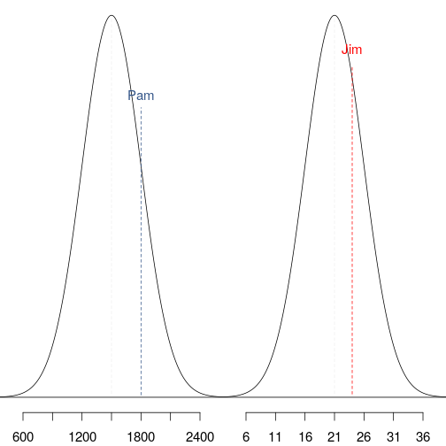
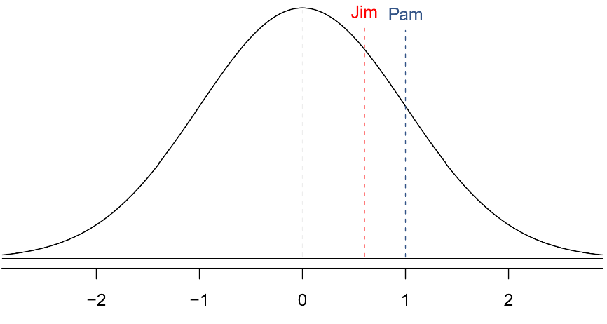
class: center, middle, inverse, title-slide # Inferential Statistics ### Thierry Warin, PhD ### quantum simulations<a style="color:#6f97d0">*</a> --- background-image: url(./images/qslogo.PNG) background-size: 100px background-position: 90% 8% # Navigation tips - Tile view: Just press O (the letter O for Overview) at any point in your slideshow and the tile view appears. Click on a slide to jump to the slide, or press O to exit tile view. - Draw: Click on the pen icon (top right of the slides) to start drawing. - Search: click on the loop icon (bottom left of the slides) to start searching. You can also click on h at any moments to have more navigations tips. --- class: inverse, center, middle # Outline --- background-image: url(./images/qslogo.PNG) background-size: 100px background-position: 90% 8% ### outline 1. Standardizing with Z scores 2. Confidence intervals --- class: inverse, center, middle # Standardizing with Z scores --- background-image: url(./images/qslogo.PNG) background-size: 100px background-position: 90% 8% # Standardizing with Z scores .pull-left[ SAT scores are distributed nearly normally with mean 1500 and standard deviation 300. ACT scores are distributed nearly normally with mean 21 and standard deviation 5. A college admissions officer wants to determine which of the two applicants scored better on their standardized test with respect to the other test takers: Pam, who earned an 1800 on her SAT, or Jim, who scored a 24 on his ACT? ] .pull-right[ <!-- --> ] --- background-image: url(./images/qslogo.PNG) background-size: 100px background-position: 90% 8% # Standardizing with Z scores .pull-left[ Since we cannot just compare these two raw scores, we instead compare how many standard deviations beyond the mean each observation is. - These are called *standardized* scores, or *Z scores*. - Z score of an observation is the number of standard deviations it falls above or below the mean. `$$Z = \frac{observation - mean}{SD}$$` - Observations that are more than 2 SD away from the mean `\(|Z| > 2\)` are usually considered unusual. ] .pull-right[ - Pam's score is `\(\frac{1800 - 1500}{300} = 1\)` standard deviation above the mean. - Jim's score is `\(\frac{24 - 21}{5} = 0.6\)` standard deviations above the mean.  ] --- class: inverse, center, middle # Confidence intervals --- background-image: url(./images/qslogo.PNG) background-size: 100px background-position: 90% 8% # Confidence intervals > A confidence interval is an interval of numbers that is likely to contain the parameter value. - A natural interval to consider is an interval centered at the sample average `\(\bar{x}\)`. The interval is set to have a width that assures the inclusion of the parameter value in the prescribed probability, namely the confidence level. The structure of the confidence interval of confidence level 95% (= *qnorm(0.975)*): `$$\bar{x} - 1.96 \times s/ \sqrt{n} \leqslant x \leqslant \bar{x} + 1.96 \times s/ \sqrt{n}$$` ```r mydata <- data.frame(stack.loss) x.bar <- mean(mydata$stack.loss) s <- sd(mydata$stack.loss) n <- length(mydata$stack.loss) ``` ```r x.bar - 1.96 * s / sqrt(n) ``` ``` ## [1] 13.17333 ``` ```r x.bar + 1.96 * s / sqrt(n) ``` ``` ## [1] 21.87428 ``` --- background-image: url(./images/qslogo.PNG) background-size: 100px background-position: 90% 8% # Confidence intervals - Suppose we took many samples and built a confidence interval from each sample using the equation: `\(point~estimate~+- 1.96 \times SE\)`. - Then about 95% of those intervals would contain the true population proportion (p). - In a confidence interval, `\(z^* \times SE\)` is called the **margin of error**, and for a given sample, the margin of error changes as the confidence level changes. - For a 95% confidence interval, `\(z^*=1.96\)`. --- class: inverse, center, middle # Conclusion --- background-image: url(./images/qslogo.PNG) background-size: 100px background-position: 90% 8% # Conclusion Inappropriate methods of sampling and data collection may produce samples that do not represent the target population. A naive application of statistical analysis to such data may produce misleading conclusions. Consequently, it is important to evaluate critically the statistical analyses we encounter before accepting the conclusions that are obtained as a result of these analyses. Common problems that occurs in data that one should be aware of include: - **Problems with Samples:** A sample should be representative of the population. A sample that is not representative of the population is biased. Biased samples may produce results that are inaccurate and not valid. - **Data Quality:** Avoidable errors may be introduced to the data via inaccurate handling of forms, mistakes in the input of data, etc. Data should be cleaned from such errors as much as possible. - **Self-Selected Samples:** Responses only by people who choose to respond, such as call-in surveys, that are often biased. - **Sample Size Issues:** Samples that are too small may be unreliable. Larger samples, when possible, are better. In some situations, small samples are unavoidable and can still be used to draw conclusions. --- background-image: url(./images/qslogo.PNG) background-size: 100px background-position: 90% 8% # Conclusion - **Undue Influence:** Collecting data or asking questions in a way that influences the response. - **Causality:** A relationship between two variables does not mean that one causes the other to occur. They may both be related (correlated) because of their relationship to a third variable. - **Self-Funded or Self-Interest Studies:** A study performed by a person or organization in order to support their claim. Is the study impartial? Read the study carefully to evaluate the work. Do not automatically assume that the study is good but do not automatically assume the study is bad either. Evaluate it on its merits and the work done. - **Misleading Use of Data:** Improperly displayed graphs and incomplete data. - **Confounding:** Confounding in this context means confusing. When the effects of multiple factors on a response cannot be separated. Confounding makes it difficult or impossible to draw valid conclusions about the effect of each factor.